

By Mark J. Anderson, Stat-Ease, Inc.
The traditional approach to experimentation—often referred to as the “scientific method”—requires changing only one factor at a time (OFAT). Unfortunately, the relatively simplistic OFAT approach falls flat when users are faced with factor or component interactions, for example, the combined impact of time and temperature on a process, or two reactants in a mixture. Because interactions abound in the coatings industry, the multifactor and multicomponent test matrices provided by the design of experiments (DOE) approach appeal greatly to process engineers and formulators.1 However, carrying out DOE correctly requires that runs be randomized whenever possible to counteract the bias that may be introduced by time-related trends, such as aging of materials, increasing humidity, and the like.
But what if complete randomization proves to be so inconvenient that it becomes impossible to run a statistically designed experiment? In this case, a specialized form of design called “split plot” becomes attractive, because of its ability to effectively group hard-to-change (HTC) factors.2 A split plot accommodates both HTC factors, for instance, the conditions in an electrostatic powder-coating chamber, and those factors that are easy to change (ETC), such as the part precleaning and preparation.
Split-plot designs originated in the field of agriculture, where experimenters applied one treatment to a large area of land, called a whole plot, and other treatments to smaller areas of land within the whole plot, called subplots. For example, Figure 1 shows two alternative experiments that were carried out on six varieties of sugar beets (Number 1 through 6) that were sown either early (E) or late (L) in the growing season:
- A completely randomized design in one field shown on the top row versus
- The bottom row where the whole plot (single field) has been split into two subplots (in this case, sown early vs late)
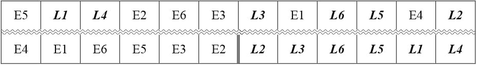
FIGURE 1—Comparing a completely randomized experiment (top row) vs one that is divided into split plots (bottom row).
The split-plot layout made it far sweeter (pun intended) for the sugar-beet farmer to sow the seeds because of the grouping, since it was far easier to plant subplots early vs late, rather than doing it in random locations.
CASE IN POINT: THE USE OF A SPLIT PLOT IN AN INDUSTRIAL EXPERIMENT
DOE pioneer George Box developed a clever experiment that led to the discovery of a highly corrosion-resistant coating for steel bars.4 Four different coatings were tested (which is easy to do) at three different furnace temperatures (which is hard to change)—each of which was run twice to provide statistical power. The design that Box pioneered (a split plot) for this experiment is shown in Table 1 (results for relative corrosion resistance—the higher the better—are shown in parentheses). Note the bars being placed at random by position.
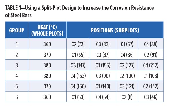
Observe in this experiment-design layout how Box made it even easier, in addition to grouping by temperature (i.e., “heats”), by increasing the furnace temperature run-by-run and then decreasing it gradually. This was done out of necessity due to the difficulties of heating and cooling a large mass of metal. The saving grace, however, is that, although shortcuts like this undermine the resulting statistics when they do not account for the restrictions in randomization, the effect estimates remain true. Thus, the results can still be assessed based on subject matter knowledge (in terms of whether they indicate important findings). Nevertheless, if possible, it will always be better to randomize levels in the whole plots and, furthermore, reset them (i.e., turn the dial away and then, after allowing time for the system to equilibrate, put it back to the same value) when they have the same value, for example, between Groups 3 and 4 in this design.
In this case, as often happens, the resetting of an HTC factor (temperature) created so much noise in this process that in a randomized design it would have overwhelmed the ability to detect the effect of the coating. The application of a split plot overcomes this variability by grouping the heats (i.e., oven batches), thus, filtering out the temperature differences. Figure 2 tells the story.
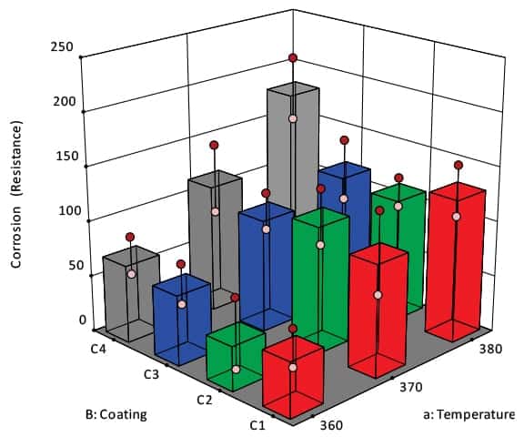
FIGURE 2—In this effects graph, 3D bars show the impact of temperature (a) vs coating (B) on corrosion resistance—the higher the better.
The best corrosion resistance occurred for coating C4 at the highest temperature (see the tallest gray tower, located at the back corner of Figure 2). This finding—the result of the two-factor interaction aB between temperature (a) and coating (B), achieved significance at p < 0.05 (that is, a level exceeding 95% confidence). The main effect of coating (B) also emerged as statistically significant. If this experiment had been run in a completely randomized way, the p-values (to put it very simply, the probability on a 0 to 1 scale of results being caused by chance) for the coating effect and the coating-temperature interaction would have been roughly 0.4 and 0.85, respectively—that is, not sufficient to be considered statistically significant. In his work, Box concludes by suggesting that coating chemists try even higher temperatures with the C4 coating while simultaneously working at better controlling the furnace temperature. Furthermore, he urges the experimenters to work at understanding better the physiochemical mechanisms causing the corrosion of the steel. This really was the genius of George Box—his matchmaking of empirical modeling tools with his subject matter expertise.
COMBINED MIXTURE-PROCESS EXPERIMENTS MADE FAR EASIER
The ability of split plots to conveniently group runs makes them especially useful for experiments that combine mixture components with process factors, for example, trying various cake recipes at varying baking conditions. Combined designs come about very commonly in the coatings industry due to the opacity being a function not only of the ingredients (mixture) but also the application (process). For example, Chau and Kelly5 studied the opacity of a printable coating material as a function of its three ingredients (two pigments and a binder) and the thickness at two levels. Figure 3 pictures the structure of this combined design—a prism. The triangular ends define the mixture—ingredients X1, X2 and X3; where the value of 1 signifies them in purest form at the apexes.6 The process factor (Z) goes from low at left to high at right, coded as -1 to +1, respectively.
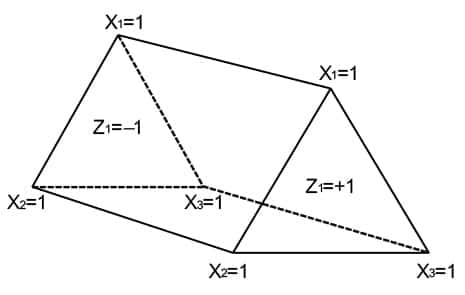
FIGURE 3—Three-component mixture combined with one process factor.
Complete randomization can be very daunting for researchers running combined designs, because:
- A new blend must be prepared, even if the recipe listed in the experimental plan does not change.
- The process must be reset, even though all the factors remain at the same level in the design.
It is not often practical, or even possible, to perform an experiment in this way. Consider, for example, a kitchen scientist mixing up a single three-ingredient cookie by the specified recipe (e.g., peanut butter, sugar, and egg) and then baking it all by itself per the process settings at time and temperature for that run. A more sensible approach would be to mix a batch of cookies and then bake a tray of them, that is, make it a split-plot experiment with components being HTC. Figure 4 lays out this experiment design.
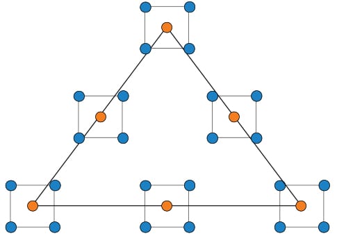
FIGURE 4—Split plot for grouping blends and then processing them.
This experiment is comprised of six master batches—three that are richest in each ingredient at the corners of the triangles, and three binary blends along the centers of the edges. The order of the batches is randomized. Each batch gets baked off at four combinations of time and temperature per a random plan.
By allowing the grouping of blends, split plots make it far easier to run statistically designed experiments on the impact of various coatings formulas on their durability under varying environmental conditions. This is just one example. Now that DOE software makes it easy to handle HTC factors or components, many situations can be managed that could not in the past due to requirements for complete randomization.
CAVEATS
Split plots essentially combine two experiment designs into one. Thus, they produce both split-plot and whole-plot random errors. For example, the corrosion-
resistance design discussed above introduces whole-plot error with each furnace re-set, due to potential variation that can result from, for instance, operator error in dialing in the temperature, inaccurate calibration, changes in ambient conditions, and so forth.7 Meanwhile, split-plot errors arise from bad measurements, variation in the distribution of heat within the furnace, differences in the thickness of the steel-bar coatings, and more.
This split-error structure creates complications in computing proper p-values for the effects, particularly when departing from a full-factorial, balanced, and replicated experiment, such as the corrosion-resistance case. If you really must use this route, be prepared for your DOE software to apply specialized statistical tools that differ from standard analysis.
Furthermore, you cannot expect that doing an experiment more conveniently will not come at a cost—nothing good comes free. The price you pay for taking advantage of split plots is the loss of power to pin down some effects on those HTC factors that are grouped, that is, not completely randomized.8
CLOSING THOUGHTS
Keep the power loss on HTC factor(s) in mind before settling for a split-plot design. Perhaps grouping HTCs for convenience may not be worth this cost—you would be better off taking the trouble to randomize the whole design. However, for many processes, running any experiment may become impossible if it requires certain factors, such as temperature, to be re-set and equilibrated for each test run; the time and expense to do this becomes prohibitive. These are situations for which a split plot can come to the rescue.
References
- Anderson, M.J. and Whitcomb, P.J., “Design of Experiments for Coatings,” Chapter 15, Coatings Technology Handbook, Third Edition, CRC Press, 15-1–15-6, 2005.
- Anderson, M.J. and Whitcomb, P.J., DOE Simplified: Practical Tools for Effective Experimentation, Third Edition, Productivity Press, Publishing, New York, NY, Chapter 11, 2015.
- Cox, D.R., Planning of Experiments, John Wiley & Sons, 1958.
- Box, G.E.P., “Split Plot Experiments,” Qual. Engin., 8(3), 515–520 (1996).
- Chau, K.W. and Kelly, W.R., “Formulating Printable Coatings via D-Optimality,” J. Coat. Technol., 65, 71-78 (June 1993).
- Anderson, M.J. and Whitcomb, P.J., “Optimization of Formulations Made Easy with Computer-Aided Design of Experiments for Mixtures,” J. Coat. Technol., 68, 71-75 (July 1996).
- Jones, B., and Nachtsheim, C., “Split-Plot Designs: What, Why, and How,” J. Qual. Technol., 41 (4), 340–361 (October 2009).
- Anderson, M.J. and Whitcomb, P.J., “Employing Power to ‘Right-Size’ Design of Experiments,” ITEA Journal, 35, 40–44 (March 2014).