
By Clifford K. Schoff, Schoff Associates
Solubility of polymers in solvents is extremely important to the coatings industry. If the solvents in a formulation are not able to dissolve the polymer or polymers to be used, either initially or during the dry or bake, the resultant film will be defective. There are two basic ways to determine solubility of polymers: trial and error, or solubility parameters. Trial and error is fine if you are trying out a new solvent, but for most situations, it is not effective.
In 1916, Hildebrand proposed that solubility could be related to the internal pressures of solvent and solute. If they were the same or nearly so, then the molecules involved would interact with each other and a solution would result. For solvents, the internal pressure can be expressed in terms of ∆E, the molar energy of vaporization, and the molar volume, V. Their ratio gives the cohesive energy density (CED). The solubility parameter is defined as
δ = (CED)1/2 = (∆E/V)1/2
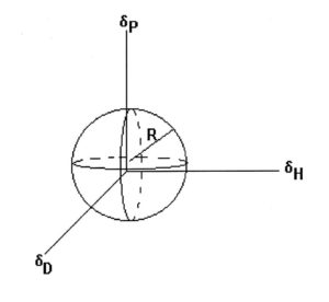
FIGURE 1—Three-dimensional solubility plot. Solvents within the sphere dissolve the polymer. Solvents outside the sphere do not dissolve it.
There are several different versions of solubility parameters, ranging from Hildebrand’s single number to various two-dimensional concepts to three-dimensions. I am most familiar with the three-dimensional system developed by Charles Hansen, which is not surprising since my first job in the coating industry was working for the same Charles Hansen. He found that ∆E arises from contributions from dispersion forces (D), polar interactions (P), and hydrogen bonding forces (H) and that three parameters, δD, δP, δH can define the solubility region of a polymer or oligomer and dissolving ability of a solvent. I have personal experience of the power of Hansen Solubility Parameters (HSP) in formulating paints and in problem solving and will give examples of their use in the next article in this series.
From a thermodynamic standpoint, solubility occurs when the free energy of mixing is negative
0 > ∆FM = ∆HM – T∆SM
Where T is the absolute temperature and ∆HM and ∆SM are the heat and entropy of mixing, respectively. The entropy term will be positive. According to Hildebrand theory, the heat of mixing is given by
∆HM = V1V2(δ1 – δ2)2
Where V1 is the volume fraction of the polymer (or other solute), V2 is the volume fraction of the solvent, δ1 is the solubility parameter of the polymer, and δ2 is the solubility parameter of the solvent. We want to minimize ∆HM because that should guarantee that the free energy of mixing, ∆FM, is negative.
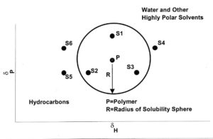
FIGURE 2—δP vs δH plots.
Considering the three parameters, we want to find the solubility region where (δD1 – δD2), (δP1 – δP2), and (δH1 – δH2) are minimized. This will define a solubility region within the δD–δP–δH space for the polymer, which encloses all the solvents that will dissolve the polymer. The region usually is represented as a sphere (see Figure 1) but may not be that regular. I have seen oblate spheroids (like an American football) and other shapes. However, treating the space as a sphere is useful in predicting the solubility of the polymer in specific solvents or blends.
Three-dimensional plots are not practical to work with, so it is common to use δP – δH plots to represent polymer solubilities and solvent parameter values. This is possible because δD values only vary over a small range. Figure 2 shows where
hydrocarbon and highly polar solvents lie on such a plot. It also shows a circle of solubility (a slice through the sphere) for a polymer. Solvents S1, S2, and S3 all are good solvents for the polymer and will dissolve it. Solvents S4, S5, and S6 are nonsolvents. However, a 1:1 mixture of S4 and S5 or S4 and S6 will dissolve the polymer because, in each case, the solubility parameter of the blend is within the circle. This is why a mixture of an alcohol and a hydrocarbon (both nonsolvents for the polymer) can dissolve that polymer.